Regression Models

---

Avisek Gupta

Indian Statistical Institute, Kolkata

---

---

Paradigms of Machine Learning:

• Supervised Learning

• Unsupervised Learning

• Reinforcement Learning

---

---

Supervised Learning Methods:

• Regression

• Classification

---

---

Regression Models

---

import numpy as np
import matplotlib.pyplot as plt

1. Linear Regression using `numpy.linalg.lstsq`

Rewriting the objective as: $\min ||X \theta - y||^2$ where the first column of $X$ is all $1$s.

# Linear Regression

data = np.array([
    [0.20, 0.30], [0.32, 0.23], [0.39, 0.35], [0.46, 0.42], 
    [0.51, 0.39], [0.60, 0.47], [0.64, 0.51], [0.75, 0.46]
])

# y = c.1 + m.x
X = np.hstack((np.ones((data.shape[0], 1)), np.reshape(data[:,0], (data.shape[0], 1))))
y = data[:,1]

theta, residual_sum, rank, s = np.linalg.lstsq(X, y, rcond=1e-9)
print(theta)
plt.figure()
plt.scatter(data[:,0], data[:,1], marker='o', c='gray')
plt.plot(
    np.array([data[:,0].min()-0.2,data[:,0].max()+0.2]), 
    theta[1] * np.array([data[:,0].min()-0.2,data[:,0].max()+0.2]) + theta[0], c='r'
)
plt.show()

2. Linear Regression using `sklearn.linear_model.LinearRegression`

• You don't need to append a column of 1s. If the Linear Regression object is created with fit_intercept=True, then it calculates the intercept.
• The Linear Regression class has variables `ceof_` and `intercept_` where the estimated parameters are stored once the model is fit on the data.

from sklearn.linear_model import LinearRegression

data = np.array([
    [0.20, 0.30], [0.32, 0.23], [0.39, 0.35], [0.46, 0.42], 
    [0.51, 0.39], [0.60, 0.47], [0.64, 0.51], [0.75, 0.46]
])

X = np.reshape(data[:,0], (data.shape[0],1))
y = data[:,1]

lr = LinearRegression(fit_intercept=True)
# X must by 2-dimensional, y must be 1-dimensional
lr.fit(X, y)
coeffs = lr.coef_
intercept = lr.intercept_
print('intercept_ =', intercept, 'coeffs_ =', coeffs)
# Score: The coefficient R^2 is defined as (1 - u/v), 
# where u is the residual sum of squares ((y_true - y_pred) ** 2).sum() 
# and v is the total sum of squares ((y_true - y_true.mean()) ** 2).sum(). 
# The best possible score is 1.0 and it can be negative 
# A constant model that always predicts the expected value of y, 
# disregarding the input features, would get a R^2 score of 0.0.
print('score =', lr.score(X, y))

plt.figure()
plt.scatter(data[:,0], data[:,1], marker='o', c='gray')
plt.plot(
    np.array([data[:,0].min()-0.2,data[:,0].max()+0.2]), 
    coeffs[0] * np.array([data[:,0].min()-0.2,data[:,0].max()+0.2]) + intercept, c='r'
)
plt.show()

3. Example of Linear Regression: Polynomial Regression

Given the data set of $(x, y)$, add linearly independent features: $x^2, x^3, ..., x^d$.

3.1. Fit the model $\mathbf{\hat{f}(x) = \theta_0 + \theta_1 x_1 + \theta_2 x_2}$

og_data = np.array([[0.2,0.3], [0.32,0.23], [0.39,0.35], [0.46, 0.42], [0.51, 0.39], [0.6, 0.47], [0.64, 0.51], [0.75, 0.46]])

x = og_data[:,0][:,None]
y = og_data[:,1]

data = np.hstack((x, x**2))

from sklearn import linear_model

reg = linear_model.LinearRegression()
reg.fit(data, y)
m, c = reg.coef_, reg.intercept_
print('m =', m, ', c =', c)
print('error =', ((reg.predict(data)- y)**2).sum())

plt.figure()
plt.scatter(data[:,0], y, marker='o', c='gray')
plt.plot(data[:,0], reg.predict(data), c='r')
plt.show()

3.2. Fit the model $\mathbf{\hat{f}(x) = \theta_0 + \theta_1 x_1 + \theta_2 x_2 + \theta_3 x_3 + \theta_4 x_4}$

og_data = np.array([[0.2,0.3], [0.32,0.23], [0.39,0.35], [0.46, 0.42], [0.51, 0.39], [0.6, 0.47], [0.64, 0.51], [0.75, 0.46]])

x = og_data[:,0][:,None]
y = og_data[:,1]

data = np.hstack((x, x**2, x**3, x**4))

from sklearn import linear_model

reg = linear_model.LinearRegression()
reg.fit(data, y)
m, c = reg.coef_, reg.intercept_
print('m =', m, ', c =', c)
print('error =', ((reg.predict(data)- y)**2).sum())

plt.figure()
plt.scatter(data[:,0], y, marker='o', c='gray')
plt.plot(data[:,0], reg.predict(data), c='r')
plt.show()

3.3. Fit the model $\mathbf{\hat{f}(x) = \theta_0 + \theta_1 x_1 + \theta_2 x_2 + \theta_3 x_3 + \theta_4 x_4 + \theta_5 x_5 + \theta_6 x_6 + \theta_7 x_7}$

og_data = np.array([[0.2,0.3], [0.32,0.23], [0.39,0.35], [0.46, 0.42], [0.51, 0.39], [0.6, 0.47], [0.64, 0.51], [0.75, 0.46]])

x = og_data[:,0][:,None]
y = og_data[:,1]

data = np.hstack((x, x**2, x**3, x**4, x**5, x**6, x**7))

from sklearn import linear_model

reg = linear_model.LinearRegression()
reg.fit(data, y)
m, c = reg.coef_, reg.intercept_
print('m =', m, ', c =', c)
print('error =', ((reg.predict(data)- y)**2).sum())

plt.figure()
plt.scatter(data[:,0], y, marker='o', c='gray')
plt.plot(data[:,0], reg.predict(data), c='r')
plt.show()

---

As model complexity increases, the training error decreases, but the generalization capabilities of the model will decreases (as indicated by the increasing test error)

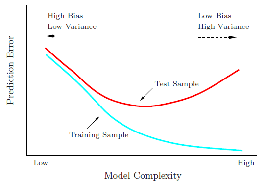
Image Source: Hastie T., Tibshirani R. & Friedman J., "The Elements of Statistical Learning", Springer New York Inc., 2001.

Remedy? The use of validation data sets to select an appropriate model complexity.

Image source: https://rpubs.com/charlydethibault/348566

---

3.4. Regression on real data sets

from sklearn.datasets import load_boston

X, y = load_boston(return_X_y=True)
print(X.shape)
print(y.shape)

from sklearn.linear_model import LinearRegression
from sklearn.datasets import load_boston

X, y = load_boston(return_X_y=True)

lr = LinearRegression(fit_intercept=True)
lr.fit(X, y)
coeffs = lr.coef_
intercept = lr.intercept_
print(intercept, coeffs)

idx = 1
plt.figure()
plt.scatter(X[:,idx], y, marker='o', c='gray')
plt.plot(
    np.array([X[:,idx].min()-0.2,X[:,idx].max()+0.2]), 
    coeffs[idx] * np.array([X[:,idx].min()-0.2,X[:,idx].max()+0.2]) + intercept, c='r'
)
plt.show()

3.5. Regression on Time Series Data

$N$ data samples are given: $y^{(i)}$ is the value at time $i=1,2,...,N$.

First download the data using the following link: Total_Petroleum_Consumption_-_World.csv

data = np.loadtxt('Total_Petroleum_Consumption_-_World.csv', delimiter=',')
# Data source: https://www.eia.gov/cfapps/ipdbproject/IEDIndex3.cfm?tid=5&pid=5&aid=2

plt.figure()
plt.plot(data[:,0], data[:,1])
plt.xlabel('Year')
plt.ylabel('Petroleum Consumption')
plt.show()

from sklearn.linear_model import LinearRegression

data = np.loadtxt('Total_Petroleum_Consumption_-_World.csv', delimiter=',')
X = np.reshape(data[:,0], (data.shape[0],1))
y = data[:,1]

lr = LinearRegression(fit_intercept=True)
lr.fit(X, y)
coeffs = lr.coef_
intercept = lr.intercept_
print(intercept, coeffs)

idx = 0
plt.figure(figsize=(12,4))
plt.subplot(121)
plt.scatter(X[:,idx], y, marker='o', c='gray')
plt.plot(
    np.array([X[:,idx].min(),X[:,idx].max()]),
    coeffs[idx] * np.array([X[:,idx].min(),X[:,idx].max()]) + intercept, c='r'
)
plt.title('Time Series Trend')

plt.subplot(122)
plt.scatter(X[:,idx], y-lr.predict(X), marker='o', c='gray')
plt.plot(np.array([X[:,idx].min(),X[:,idx].max()]), np.array([0,0]), c='#000099', linestyle='--')
plt.title('De-trended Time Series')

plt.show()

3.6. Time Series with periodic components

First download the data using the following link: us_vehicle_data.csv

data = np.loadtxt('us_vehicle_data.csv', delimiter=',')
# Data source: https://fred.stlouisfed.org/series/TRFVOLUSM227NFWA

plt.figure(figsize=(10,4), dpi=200)
plt.plot(np.arange(data.shape[0]), data[:,1])
plt.xticks(np.arange(0, data.shape[0], data.shape[0]//13), np.arange(2004,2018+1))
plt.xlabel('Year')
plt.ylabel('Distance (in miles)')
plt.show()

The Regression model $\hat{y} = \hat{y}^{lin} + \hat{y}^{seas}$, we estimate: $(\theta_1, \theta_2, ..., \theta_{P+1})$

$\theta_1$ : For the linear part, $\hat{y}^{lin} = \theta_1 \begin{bmatrix}1 \\ 2 \\ \vdots \\ N \end{bmatrix}$

$\theta_2$ to $\theta_{P+1}$ : For the $P$ periodic components, $\hat{y}^{seas} = (y_2, ..., y_{N})$, where, $\hat{y_i} = I_{P} \theta_{i}$

The problem becomes: $\min\limits_{theta} ||A \theta - y ||^2$, where, $A_{1:N,1} = \begin{bmatrix}1 \\ 2 \\ \vdots \\ N \end{bmatrix}$, $A_{1:N,2:P+1} = \begin{bmatrix} I_{P} \\ I_{P} \\ \vdots \\ I_{P} \end{bmatrix}$, $y = \begin{bmatrix} y_1 \\ y_2 \\ \vdots \\ y_N \end{bmatrix}$

from sklearn.linear_model import LinearRegression

data = np.loadtxt('us_vehicle_data.csv', delimiter=',')
X1 = np.arange(data.shape[0])+1
X2 = []
for iter1 in range(data.shape[0]//12):
    if iter1 == 0:
        X2 = np.eye(12)
    else:
        X2 = np.vstack((X2, np.eye(12)))
X = np.hstack((np.reshape(X1, (X1.shape[0],1)), X2))
print(X.shape)
y = data[:,1]

lr = LinearRegression(fit_intercept=True)
lr.fit(X, y)
coeffs = lr.coef_
intercept = lr.intercept_
print(intercept, coeffs)

plt.figure(figsize=(10,4), dpi=200)
plt.scatter(np.arange(data.shape[0]), data[:,1], c='w', edgecolor='g')
plt.plot(np.arange(data.shape[0]), lr.predict(X))
plt.xticks(np.arange(0, data.shape[0], data.shape[0]//13), np.arange(2004,2018+1))
plt.xlabel('Year')
plt.ylabel('Distance (in miles)')
plt.show()

4. Ridge Regression

$\mathbf{\min\limits_{w} ||Xw - y||_{2}^2 + \alpha ||w||_{2}^2}$

# Author: Kornel Kielczewski -- <kornel.k@plusnet.pl>

print(__doc__)

import matplotlib.pyplot as plt
import numpy as np

from sklearn.datasets import make_regression
from sklearn.linear_model import Ridge
from sklearn.metrics import mean_squared_error

clf = Ridge()

X, y, w = make_regression(n_samples=10, n_features=10, coef=True,
                          random_state=1, bias=3.5)

coefs = []
errors = []

alphas = np.logspace(-6, 6, 200)

# Train the model with different regularisation strengths
for a in alphas:
    clf.set_params(alpha=a)
    clf.fit(X, y)
    coefs.append(clf.coef_)
    errors.append(mean_squared_error(clf.coef_, w))

# Display results
plt.figure(figsize=(20, 6))

plt.subplot(121)
ax = plt.gca()
ax.plot(alphas, coefs)
ax.set_xscale('log')
plt.xlabel('alpha')
plt.ylabel('weights')
plt.title('Ridge coefficients as a function of the regularization')
plt.axis('tight')

plt.subplot(122)
ax = plt.gca()
ax.plot(alphas, errors)
ax.set_xscale('log')
plt.xlabel('alpha')
plt.ylabel('error')
plt.title('Coefficient error as a function of the regularization')
plt.axis('tight')

plt.show()

og_data = np.array([[0.2,0.3], [0.32,0.23], [0.39,0.35], [0.46, 0.42], [0.51, 0.39], [0.6, 0.47], [0.64, 0.51], [0.75, 0.46]])

x = og_data[:,0][:,None]
y = og_data[:,1]

data = np.hstack((x, x**2, x**3, x**4))

from sklearn.linear_model import LinearRegression
from sklearn.linear_model import Ridge

reg1 = LinearRegression()
reg1.fit(data, y)
m, c = reg1.coef_, reg1.intercept_
print('m =', m, ', c =', c)
print('error =', ((reg1.predict(data)- y)**2).sum())

plt.figure()
plt.scatter(data[:,0], y, marker='o', c='gray')
plt.plot(data[:,0], reg1.predict(data), c='r')
plt.show()

reg2 = Ridge(alpha=0.05)
reg2.fit(data, y)
m, c = reg2.coef_, reg2.intercept_
print('m =', m, ', c =', c)
print('error =', ((reg2.predict(data)- y)**2).sum())

plt.figure()
plt.scatter(data[:,0], y, marker='o', c='gray')
plt.plot(data[:,0], reg2.predict(data), c='r')
plt.show()

5. Lasso Regression

$\mathbf{\min\limits_{w} ||Xw - y||_{2}^2 + \alpha ||w||_{1}}$

import numpy as np

from sklearn.datasets import make_regression
from sklearn.linear_model import Lasso

X, y, w = make_regression(n_samples=10, n_features=10, coef=True,
                          random_state=1, bias=3.5)

clf = Lasso()

alphas = np.linspace(0.1, 40, 200)

zero_w = []
for a in alphas:
    clf.set_params(alpha=a)
    clf.fit(X, y)
    zero_w.append(np.sum(clf.coef_==0))
    
plt.figure(dpi=90)
plt.plot(alphas, zero_w)
plt.xlabel('alpha')
plt.ylabel('# zero features')
plt.axis('tight')
plt.show()