Supervised Learning: Classification
Avisek Gupta
Indian Statistical Institute, Kolkata
1. Simple Gradient Descent, with adaptive step size (Using backtracking line search)
import numpy as np

def fun1(x):
    return (x-1)**2 + 4

def grad_fun1(x):
    return 2*(x-1)

def gradient_descent(fun, grad, x0, max_iter=1000, tol=1e-12):
    x_prev = x0
    f_prev = fun(x_prev)

    list_x = [x0]
    alpha = 10
    for iter1 in range(max_iter):
        while 1:
            x_new = x_prev - alpha * grad(x_prev)
            f_new = fun(x_new)
            if f_new >= f_prev:
                alpha /= (iter1+2)
            else:
                break
        if (f_new - f_prev)**2 < tol:
            print('Terminating after iteration', iter1)
            break
        f_prev = f_new
        x_prev = x_new
        list_x.append(x_new)
    return x_new, list_x

x0 = np.random.rand()*20-10
print('Initial Guess =', x0)
print('Initial Objective Function Value =', fun1(x0))
print('')

soln, list_x = gradient_descent(fun=fun1, grad=grad_fun1, x0=x0)
print('Solution =', soln)
print('Final Objective Function Value =', fun1(soln))

import matplotlib.pyplot as plt
x = np.linspace(-10, 10, 100)
plt.plot(x, fun1(x), c='gray')
plt.scatter(list_x, fun1(np.array(list_x)), c='r', marker='x')
plt.show()

2. Gradient Descent using the minimize function present under scipy.optimize
import numpy as np
from scipy.optimize import minimize

def fun1(x):
    return x**2 + 4

def grad_fun1(x):
    return 2*x

x0 = np.random.randint(1,100)
print('Initial Guess =', x0)

res = minimize(fun=fun1, jac=grad_fun1, x0=x0, method='Newton-CG')

print(res)
print('---------------------')
print('Success?', res.success)
print('Solution =', res.x)
print('Objective Function Value =', res.fun)
3. Perceptron
For 2-class Classification:
$f(x) = \begin{cases} 1 & \text{ if } w^T x + b > 0 \\ -1 & \text{ otherwise} \end{cases} $
a1 = np.random.uniform(low=0, high=0.5, size=(100,2))
a2 = np.random.uniform(low=0.5, high=1, size=(100,2))

X = np.hstack((np.ones((200,1)), np.vstack((a1, a2))))
y = np.hstack(( np.zeros((100))-1, np.ones((100)) ))

plt.scatter(a1[:,0], a1[:,1], marker='x')
plt.scatter(a2[:,0], a2[:,1], marker='x')

plt.show()

The Perceptron Learning Rule :
$ w^{(t+1)} = w^{(t)} - \alpha.\frac{1}{n} \sum\limits_{i=1}^{n} ( y_i - f(x_i)). x_i$
w = np.random.rand(X.shape[1]) * 2 - 1
print(w)

plt.scatter(X[:,1], X[:,2], marker='x', c='gray')
extreme_xvals = np.array([np.min(X[:,1]), np.max(X[:,1])])
plt.plot(extreme_xvals, (-w[0] - w[1] * extreme_xvals) / w[2], c='r')
plt.show()

for iter1 in range(300):
    w += 0.1 * np.mean((y - np.sign(np.dot(X, w)))[:,None] * X, axis=0)
print(w)

plt.scatter(X[:,1], X[:,2], marker='x', c='gray')
plt.plot(extreme_xvals, (-w[0] - w[1] * extreme_xvals) / w[2], c='r')
plt.ylim(extreme_xvals)
plt.show()


An Objective Function for the Perceptron
$\min \sum\limits_{i : f(x_i) \neq y_i} -y_i (w^T x_i) $
Gradient of the Objective Function :
$\sum\limits_{i : f(x_i) \neq y_i} -y_i x_i $
def obj_fun(w):
    idx = y != np.sign(np.dot(X, w))
    return np.sum(-y[idx] * np.dot(X[idx,:], w))

def obj_grad(w):
    idx = y != np.sign(np.dot(X, w))
    return np.sum((-y[idx][:,None] * X[idx,:]), axis=0)

def gradient_descent(fun, grad, x0, max_iter=300, tol=1e-12):
    x_prev = x0
    f_prev = fun(x_prev)

    list_x = [x0]
    alpha = 0.1
    for iter1 in range(max_iter):
        x_new = x_prev - alpha * grad(x_prev)
        f_new = fun(x_new)
        #print(f_new)
        if (f_new - f_prev)**2 < tol:
            print('Terminating after iteration', iter1)
            break
        f_prev = f_new
        x_prev = x_new
        list_x.append(x_new)
    return x_new, list_x

w0 = np.random.rand(X.shape[1]) * 2 - 1
print('Initial Guess =', w0)
print('Initial Obj Fun Val =', obj_fun(w0))

plt.scatter(X[:,1], X[:,2], marker='x', c='gray')
extreme_xvals = np.array([np.min(X[:,1]), np.max(X[:,1])])
plt.plot(extreme_xvals, (-w0[0] - w0[1] * extreme_xvals) / w0[2], c='r')
#plt.ylim(extreme_xvals)
plt.show()

final_w, list_w = gradient_descent(fun=obj_fun, grad=obj_grad, x0=w0)
print('Final w =', final_w)
print('Final Obj Fun Val =', obj_fun(final_w))

plt.scatter(X[:,1], X[:,2], marker='x', c='gray')
plt.plot(extreme_xvals, (-final_w[0] - final_w[1] * extreme_xvals) / final_w[2], c='r')
plt.ylim(extreme_xvals)
plt.show()


3.1. Gradient Descent on Perceptrons using the scipy.optimize.minimize function
def obj_fun(w):
    idx = y != np.sign(np.dot(X, w))
    return np.sum(-y[idx] * np.dot(X[idx,:], w))

def obj_grad(w):
    idx = y != np.sign(np.dot(X, w))
    return np.sum((-y[idx][:,None] * X[idx,:]), axis=0)


w0 = np.random.rand(X.shape[1]) * 2 - 1
print('Initial Guess =', w0)
print('Initial Obj Fun val =', obj_fun(w0))

plt.scatter(X[:,1], X[:,2], marker='x', c='gray')
extreme_xvals = np.array([np.min(X[:,1]), np.max(X[:,1])])
plt.plot(extreme_xvals, (-w0[0] - w0[1] * extreme_xvals) / w0[2], c='r')
plt.show()

res = minimize(fun=obj_fun, jac=obj_grad, x0=w0, method='CG')
print(res.success)

plt.scatter(X[:,1], X[:,2], marker='x', c='gray')
final_w = res.x
print('Final w =', final_w)
print('Obj Fun val =', obj_fun(final_w))
plt.plot(extreme_xvals, (-final_w[0] - final_w[1] * extreme_xvals) / final_w[2], c='r')
plt.ylim(extreme_xvals+np.array([-0.05, 0.05]))
plt.show()


4. Logistic Regression
The objective function:
$\max \frac{1}{n} \sum\limits_{i=1}^{n} \{ y_i \log g(x_i) + (1 - y_i) \log (1 - g(x_i)) \} $, where $g(x_i) = \frac{1}{1+\exp(-w^T x_i)}$
The gradient of the objective function is:
$-\frac{1}{n} \sum\limits_{i=1}^{n} (y_i - g(x_i))x_i$
X = np.hstack((np.ones((200,1)), np.vstack((a1, a2))))
y = np.hstack(( np.zeros((100)), np.ones((100)) ))

def obj_fun(w):
    gx = 1 / (1 + np.exp(-np.dot(X, w)))
    return -np.mean(y * np.log(np.fmax(gx, 1e-6)) + (1 - y) * np.log(np.fmax(1 - gx, 1e-6)))

def obj_grad(w):
    gx = 1 / (1 + np.exp(-np.dot(X, w)))
    return -np.mean(np.reshape(y - gx, (y.shape[0],1)) * X, axis=0)


w0 = np.random.rand(X.shape[1]) * 2 - 1
print('Initial Guess =', w0)
print('Initial Obj Fun val =', obj_fun(w0))

plt.figure()
plt.scatter(X[:,1], X[:,2], marker='x', c='gray')
extreme_xvals = np.array([np.min(X[:,1]), np.max(X[:,1])])
plt.plot(extreme_xvals, (-w0[0] - w0[1] * extreme_xvals) / w0[2], c='r')
plt.show()

res = minimize(fun=obj_fun, jac=obj_grad, x0=w0, method='CG')
print(res.success)

plt.figure()
plt.scatter(X[:,1], X[:,2], marker='x', c='gray')
final_w = res.x
print('Final w =', final_w)
print('Obj Fun val =', obj_fun(final_w))
plt.plot(extreme_xvals, (-final_w[0] - final_w[1] * extreme_xvals) / final_w[2], c='r')
plt.ylim(extreme_xvals+np.array([-0.05, 0.05]))
plt.show()


A visual depiction of the change in function values as we move away from the decision boundary. The same color indicates the same value of $f(x_i)$.
tx, ty = np.meshgrid(
    np.linspace(0,1,100),
    np.linspace(0,1,100)
)
plot_data = np.hstack((
    np.ones((tx.shape[0]**2,1)), np.hstack((
        np.reshape(tx, (tx.shape[0]**2,1)),
        np.reshape(ty, (ty.shape[0]**2,1))
    ))
))

plot_pred = 1 / (1 + np.exp(-np.dot(plot_data, final_w)))

plt.figure()
plt.scatter(plot_data[:,1], plot_data[:,2], marker='o', c=plot_pred, cmap='Reds')
final_w = res.x
print('Final w =', final_w)
print('Obj Fun val =', obj_fun(final_w))
plt.show()

5. Support Vector Machines
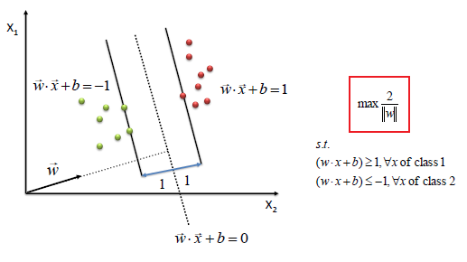
Image source: http://www.saedsayad.com/support_vector_machine.htm
Objective:
$\max \dfrac{2}{||w||}$
Subject to, $y_i(w^Tx_i+b) \geq 1$
Reformulated Optimization Problem:
$\max W(\alpha) = \sum\limits_{i=1}^{n} \alpha_i - \frac{1}{2} \sum\limits_{i,j=1}^{n} y_i y_j \alpha_i \alpha_j x_i^T x_j $
Subject to, $\alpha_i \geq 0\ \ \forall i$
$\sum\limits_{i=1}^{n} \alpha_i y_i = 0$
From the solution of the above problem, we can calculate the parameters
$w = \sum\limits_{i=1}^{n} \alpha_i y_i x_i$
$b = -\dfrac{\max\limits_{i:y_i=-1} w^T x_i\ +\ \min\limits_{i:y_i=1} w^T x_i}{2}$
from sklearn.datasets import make_blobs
X, y = make_blobs(n_samples=100, n_features=2, centers=2)
y[y==0] = -1
X = np.hstack((np.ones((X.shape[0],1)), X))
gram = np.dot(X, X.T)

plt.figure(figsize=(8,6))
for iter1 in np.unique(y):
    plt.scatter(X[y==iter1,1], X[y==iter1,2])
plt.xlabel('Feature 1')
plt.ylabel('Feature 2')
plt.title('2 classes of random data', size=16)
plt.axis('tight')
plt.show()

We will use the `SLSQP' solver in svm.optimize.minimize, which can be used for constrained optimization problems.
def svm_obj(a, y, gram):
    ya = y * a
    return 0.5 * np.sum(np.outer(ya, ya)* gram) - np.sum(a)

def svm_grad(a, y, gram):
    ya = y * a
    return 0.5 * y * np.sum(ya*gram, axis=1) - 1

cons = (
    {'type': 'eq',
    'fun':  lambda alpha, y: np.dot(alpha, y),
    'jac':  lambda alpha, y: y,
    'args': (y, )}
)

a0 = np.random.rand(X.shape[0]) * 2 - 1
res = minimize(
    fun=svm_obj,
    jac=svm_grad,
    x0=a0,
    args=(y, gram),
    constraints=cons,
    bounds=[(0, 1000) for _ in range(X.shape[0])],
    method='SLSQP'
)

#print(res)
w = np.zeros((X.shape[1]))
w[1:] = np.sum((res.x * y)[:,None] * X[:,1:], axis=0)
w[0] = -0.5 * (np.max(np.dot(X[y==-1,1:], w[1:])) + np.min(np.dot(X[y==1,1:], w[1:])))
print(w)

plt.figure()
plt.scatter(X[:,1], X[:,2], marker='x', c='gray')
extreme_xvals = np.array([np.min(X[:,1]), np.max(X[:,1])])
plt.plot(extreme_xvals, (-w[0] - w[1] * extreme_xvals) / w[2], c='r')
plt.show()

Plots of the classified data and the maximal margin
plt.figure(figsize=(8,6))
plt.clf()
plt.scatter(
    X[:, 1], X[:, 2], c=y, zorder=10,
    cmap=plt.cm.Paired, edgecolor='k', s=20
)
plt.axis('tight')
x_min = X[:, 1].min()
x_max = X[:, 1].max()
y_min = X[:, 2].min()
y_max = X[:, 2].max()
XX, YY = np.mgrid[x_min:x_max:200j, y_min:y_max:200j]
Z = np.dot(np.hstack((np.ones((XX.shape[0]**2,1)), np.hstack((XX.ravel()[:,None], YY.ravel()[:,None])) )), w)

# Put the result into a color plot
Z = Z.reshape(XX.shape)
plt.pcolormesh(XX, YY, Z > 0, cmap=plt.cm.Paired)
plt.contour(XX, YY, Z, colors=['k', 'k', 'k'],
            linestyles=['--', '-', '--'], levels=[-1, 0, 1])
plt.xlabel('Feature 1')
plt.ylabel('Feature 2')
plt.title('Linear SVM', size=20)
plt.show()
# ~~~~~~~~~~~~~~~~~~~~~~~~~~ #
