2D bent-straight waveguide couplers simulator

|
2D bent-straight waveguide couplers simulator |
|
Bent-straight waveguide couplers are one of the ingredients of the "standard model" of circular microresonators. The response of these couplers is characterized by scattering matrices, which in turn determine the spectral response of the resonators. Therefore it is essential to have a parameter free model of bent-straight waveguide couplers.
Capitalizing on the availability of rigorous analytical modal solutions for 2-D bent waveguides, these couplers are modeled using a frequency domain spatial coupled mode formalism, derived by means of a variational principle or reciprocity technique.
Here, we analyze the interaction between bent waveguides and straight waveguides in two dimensional settings, using spatial coupled mode theory. The formulation presented in here takes into account that multiple modes in each of the cores may turn out to be relevant for the functioning of the resonators. Having access to analytical 2-D bend modes proves useful for the numerical implementation of this model.
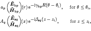
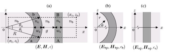
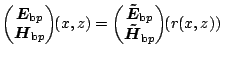
Consider the coupler configuration shown in Figure 1(a). The coupled mode theory description starts with the
specification of the basis fields, here the time-harmonic modal solutions associated with
the isolated bent (b) and straight cores (c). Customarily, the real, positive
frequency ![]() is given by the vacuum wavelength
is given by the vacuum wavelength ![]() ;
we omit the common time dependence
;
we omit the common time dependence
![]() for the sake of brevity. Only forward propagating modes are considered, where,
for convenience, we choose the
for the sake of brevity. Only forward propagating modes are considered, where,
for convenience, we choose the ![]() -axis of the Cartesian system as introduced
in Figure 1 as the common propagation coordinate
for all fields.
-axis of the Cartesian system as introduced
in Figure 1 as the common propagation coordinate
for all fields.
 |
Let
![]() ,
,
![]() , and
, and
![]() represent the modal electric fields, magnetic fields, and the spatial
distribution of the relative permittivity of the bent waveguide. Due to the
rotational symmetry, these fields are naturally given in the polar coordinate
system
represent the modal electric fields, magnetic fields, and the spatial
distribution of the relative permittivity of the bent waveguide. Due to the
rotational symmetry, these fields are naturally given in the polar coordinate
system ![]() ,
, ![]() associated with the bent waveguide. For the application
in the CMT formalism, the polar coordinates are expressed in the Cartesian
associated with the bent waveguide. For the application
in the CMT formalism, the polar coordinates are expressed in the Cartesian
![]() -
-![]() -system, such that the basis fields for the cavity read
-system, such that the basis fields for the cavity read
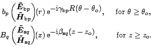
Likewise,
![]() ,
,
![]() , and
, and
![]() denote the modal fields and the relative permittivity
associated with the straight waveguide. These are of the form
denote the modal fields and the relative permittivity
associated with the straight waveguide. These are of the form
Now the total optical electromagnetic field
![]() ,
,
![]() inside the
coupler region is assumed to be well represented by a linear combination of
the modal basis fields (1), (2),
inside the
coupler region is assumed to be well represented by a linear combination of
the modal basis fields (1), (2),
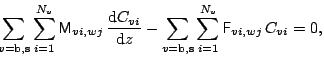
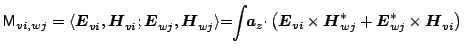
For the further procedures, the unknown coefficients ![]() are combined
into amplitude vectors
are combined
into amplitude vectors
![]() . By using a variational principle or
Lorentz reciprocity theorem, one gets the following coupled mode equation for
these unknowns (see Ref. [2])
. By using a variational principle or
Lorentz reciprocity theorem, one gets the following coupled mode equation for
these unknowns (see Ref. [2])
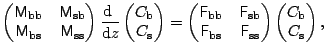
In matrix notation, equations (4) read
In the single mode case
![]() , Eq.(7) is
given explicitely [3, 4] as
, Eq.(7) is
given explicitely [3, 4] as
 |
(8) |
To proceed further, the coupled mode equations are solved by
numerical means; the result
can be stated in terms of a transfer matrix
T that relates the CMT
amplitudes at the output plane
![]() to the amplitudes at the
input plane
to the amplitudes at the
input plane
![]() of the coupler region:
of the coupler region:
For a typical coupler configuration, the guided modal fields of the
straight waveguide are well confined to the straight core. On the contrary,
due to the radiative nature of the fields, the bend mode profiles can extend
far beyond the outer interface of the bent waveguide. Depending upon the
specific physical configuration, the extent of these radiative parts of the
fields varies, such that also outside the actual coupler region, the field
strength of the bend modes in the region close to the straight core may be
significant. Therefore, to assign the external mode amplitudes ![]() ,
, ![]() , it turns out to be necessary
to project the coupled field on the straight waveguide modes.
, it turns out to be necessary
to project the coupled field on the straight waveguide modes.
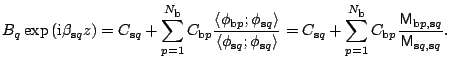
At a sufficient distance from the cavity, in the region where only the
straight waveguide is present, the total field
![]() can be expanded into the complete set of modal
solutions of the eigenvalue problem for the straight waveguide. The basis
set consists of a finite number of guided modes
can be expanded into the complete set of modal
solutions of the eigenvalue problem for the straight waveguide. The basis
set consists of a finite number of guided modes
![]() and a nonguided,
radiative part
and a nonguided,
radiative part
![]() , such that
, such that
 |
(12) |
Thus, given the solution (9) of the coupled mode equations in the form
of the transfer matrix
T, the scattering matrix
S that
relates the amplitudes ![]() ,
, ![]() ,
, ![]() ,
, ![]() of the external fields
(shown in Figure 1) is defined as
of the external fields
(shown in Figure 1) is defined as
A lower left block is filled with entries
![]() and
and
![]() ,
for
,
for
![]() and
and
![]() ,
respectively, that incorporate the projections.
All other coefficients of
P and
Q are zero.
,
respectively, that incorporate the projections.
All other coefficients of
P and
Q are zero.
Go to top
The coupled mode equations (4), (7)
are treated by numerical means on a rectangular computational window
![]() as
introduced in Figure 1. The solution involves the
numerical quadrature of the integrals (5), (6) in the
as
introduced in Figure 1. The solution involves the
numerical quadrature of the integrals (5), (6) in the
![]() -dependent matrices
M and
F, where a simple trapezoidal
rule [5] is applied, using an equidistant discretization of
-dependent matrices
M and
F, where a simple trapezoidal
rule [5] is applied, using an equidistant discretization of
![]() into intervals of length
into intervals of length ![]() .
.
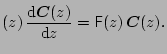
Subsequently, a standard fourth order Runge-Kutta scheme [5] serves
to generate a numerical solution of the coupled mode equations
over the computational domain
![]() , which is split
into intervals of equal length
, which is split
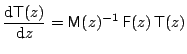
into intervals of equal length ![]() . Exploiting the linearity of equation
(7), the procedure is formulated directly for the transfer matrix
T, i.e. applied to the matrix equation
. Exploiting the linearity of equation
(7), the procedure is formulated directly for the transfer matrix
T, i.e. applied to the matrix equation
 |
(15) |
As a result, one gets the required transfer matrix T. By incorporating the projections, then it leads to the required scattering matrix S.
| bscoupler.h, bscoupler.c | Bent-straight waveguide coupler (More) |
Couplers simulator: Example
K. R. Hiremath, M. Hammer, S. Stoffer, L. Prkna, and J. Ctyroký.
Analytic approach to dielectric optical bent slab waveguides.
Optical and Quantum Electronics, 37(1-3):37-61, January 2005.
K. R. Hiremath, R. Stoffer, and M. Hammer.
Modeling of circular integrated optical microresonators by 2-D
frequency domain coupled mode theory.
2005.
(accepted).
R. Stoffer, K. R. Hiremath, and M. Hammer.
Comparison of coupled mode theory and FDTD simulations of coupling
between bent and straight optical waveguides.
In M. Bertolotti, A. Driessen, and F. Michelotti, editors, Microresonators as building blocks for VLSI photonics, volume 709 of AIP
conference proceedings, pages 366-377. American Institute of Physics,
Melville, New York, 2004.
M. Hammer, K. R. Hiremath, and R. Stoffer.
Analytical approaches to the description of optical microresonator
devices.
In M. Bertolotti, A. Driessen, and F. Michelotti, editors, Microresonators as building blocks for VLSI photonics, volume 709 of AIP
conference proceedings, pages 48-71. American Institute of Physics,
Melville, New York, 2004.
W. H. Press, S. A. Teukolsky, W. T. Vetterling, and B. P. Flannery.
Numerical Recipes in C, 2nd ed.
Cambridge University Press, 1992.
|
|

|

|
|

|
 e
e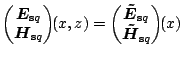 e
e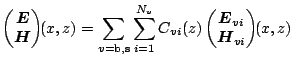
 d
d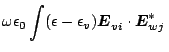 d
d